Traitement du signal

Jean-Yves Tourneret, Charly Poulliat

Bibliographie

• J. Max et J.-L. Lacoume, Méthodes et techniques de traitement du signal, Dunod, \(5\)ème édition, \(2004\).

• Athanasios Papoulis and S. Unnikrishna Pillai, Probability, Random Variables and Stochastic Processes}, McGraw Hill Higher Education, \(4\)th edition, 2002.

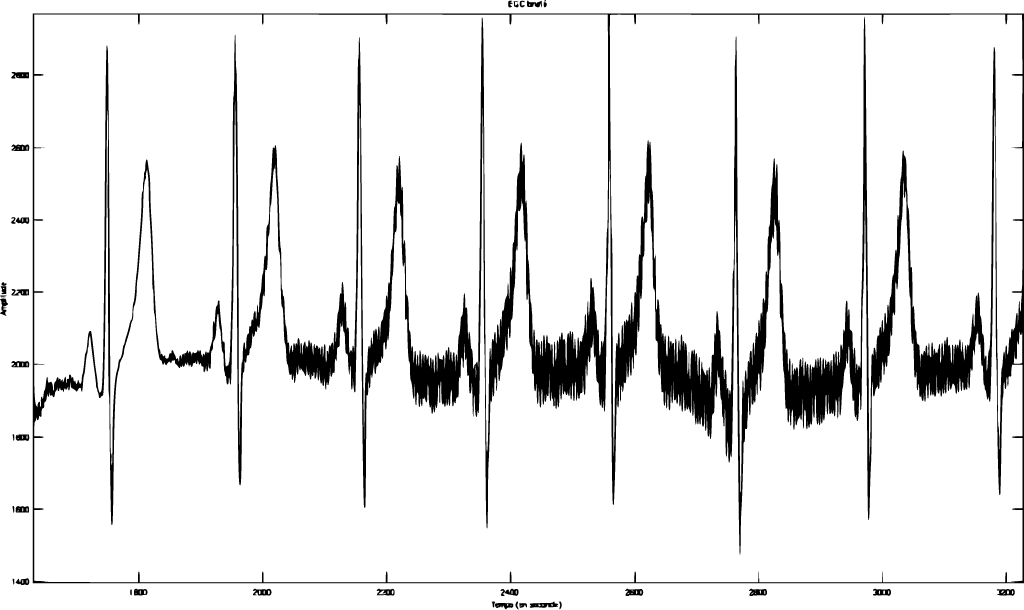
Electrocardiogramme

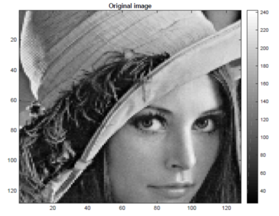
Lena

Plan du cours

• Chapitre 1 : Corrélations et Spectres

• Chapitre 2 :Filtrage Linéaire

• Chapitre 3 : Traitements Non-linéaires

Plan du cours

• Chapitre 1 : Corrélations et Spectres

  • Transformée de Fourier
  • Classes de signaux déterministes et aléatoires
  • Propriétés de \(R_x(\tau)\) et de \(s_x(f)\)

• Chapitre 2 :Filtrage Linéaire

• Chapitre 3 : Traitements Non-linéaires

Transformée de Fourier

• Définitions

  • Formule directe

  \[X(f)=\int_{\mathbb{R}} x(t) \exp \left( - j 2 \pi ft \right) dt\]

  • Formule inverse

  \[x(t)=\int_{\mathbb{R}} X(f) \exp \left( j 2 \pi ft \right) df\]

• Hypothèses : TF sur \(\mathcal{L}^1\) ou \(\mathcal{L}^2\)

Propriétés

• Linéarité \[\textrm{TF} \left[a x(t)+ by(t) \right] = a X(f) + bY(f)\]

• Parité : \(x(t)\) réelle paire \(\Rightarrow\) \(X(f)\) réelle paire

• Translation et Modulation : \[\begin{align*} &\textrm{TF} \left[x(t-t_0) \right] = \exp (-j2 \pi f t_0) X(f)\\ &\textrm{TF} \left[x(t) \exp (j 2 \pi f_0 t)\right]=X(f-f_0) \end{align*}\]

• Similitude :

\[\textrm{TF} \left[x(at) \right] = \frac{1}{|a|} X \left(\frac{f}{a}\right)\]

Propriétés

• Produit de convolution :

  • Définition

  \[\begin{aligned} y(t)=(h * x)(t)=h(t)*x(t)&= \int_{-\infty}^{\infty} x(\tau) h(t-\tau) d \tau \\ &=\int_{-\infty}^{\infty} x(t-\tau) h(\tau) d \tau \end{aligned}\]

  • TF

\[\begin{aligned} &\textrm{TF} \left[ x(t) * y(t) \right] = X(f) Y(f)\\ &\textrm{TF} \left[ x(t) y(t) \right] = X(f) * Y(f) \end{aligned}\]

• Egalité de Parseval :

\[ \int_{\mathbb{R}} x(t) y^*(t) dt = \int_{\mathbb{R}} X(f) Y^*(f) df \]

Distributions

• Localisation :

\[x(t) \delta(t-t_0) = x(t_0) \delta(t-t_0)\]

• Produit de Convolution :

\[x(t) * \delta(t-t_0) = x(t-t_0)\]

• Transformées de Fourier :

\[\begin{aligned} &\textrm{TF} \left[ \delta(t) \right] = 1, \; \textrm{TF} \left[ 1 \right] = \delta(f)\\ &\textrm{TF} \left[ \delta(t-t_0) \right] = \exp (- j 2 \pi f t_0), \; \textrm{TF} \left[ \exp (j 2 \pi f_0 t) \right] = \delta(f-f_0) \end{aligned}\]

Résumé des propriétés

\[\begin{array}{|ccc|} \hline & \textbf{T.F.} & \\ \hline ax(t)+by(t) &\rightleftharpoons & aX(f)+bY(f) \\ \hline x(t-t_{0}) & \rightleftharpoons & X(f)e^{-i2\pi ft_{0}} \\ \hline x(t)e^{+i2\pi f_{0}t} & \rightleftharpoons & X(f-f_{0}) \\ \hline x^{\ast }(t) & \rightleftharpoons & x^{\ast }(-f) \\ \hline x(t)~.~y(t) & \rightleftharpoons & X(f)\ast Y(f) \\ \hline x(t)\ast y(t) & \rightleftharpoons & X(f)~.~Y(f) \\ \hline x(at+b) & \rightleftharpoons & \frac{1}{\left| a\right| }X\left( \frac{f}{a}\right) e^{i2\pi \frac{b}{a}f}\\ \hline \frac{dx^{(n)}(t)}{dt^{n}} & \rightleftharpoons & \left( i2\pi f\right) ^{n}X(f) \\ \hline \left( -i2\pi t\right) ^{n}x(t) & \rightleftharpoons & \frac{dX^{(n)}(f)}{df^{n}} \\ \hline \end{array}\]

\[\begin{array}{|c|c|} \hline\hline \textbf{Formule de Parseval} & \textbf{Série de Fourier} \\ \hline\hline \int_{\mathbb{R}}x(t)y^{\ast }(t)dt=\int_{\mathbb{R}}X(f)Y^{\ast }(f)df & \underset{n\in \mathbb{Z}}{\sum }c_{n}e^{+i2\pi nf_{0}t}\rightleftharpoons \underset{n\in \mathbb{Z}}{\sum }c_{n}\delta \left( f-nf_{0}\right) \\ \hline \int_{\mathbb{R}}\left| x(t)\right| ^{2}dt=\int_{\mathbb{R}}\left| X(f)\right| ^{2}df & \\ \hline \end{array}\]

Tables

\[\begin{array}{|ccc|} \hline & \textbf{T.F.} & \\ \hline 1 & \rightleftharpoons & \delta \left( f\right)\\ \hline \delta \left( t\right) & \rightleftharpoons & 1 \\ \hline e^{+i2\pi f_{0}t} & \rightleftharpoons & \delta \left( f-f_{0}\right) \\ \hline \delta \left( t-t_{0}\right) & \rightleftharpoons& e^{-i2\pi ft_{0}} \\ \hline \amalg \hspace{-0.2cm}\amalg _{T}\left( t\right) =\underset{k\in \mathbb{Z}}{\sum }\delta \left( t-kT\right) & \rightleftharpoons & \frac{1}{T}\amalg \hspace{-0.2cm} \amalg _{1/T}\left( f\right) \\ \hline \cos \left( 2\pi f_{0}t\right) & \rightleftharpoons & \frac{1}{2}\left[ \delta \left( f-f_{0}\right)+\delta \left( f+f_{0}\right) \right] \\ \hline \sin \left( 2\pi f_{0}t\right) & \rightleftharpoons & \frac{1}{2i}\left[ \delta \left( f-f_{0}\right)-\delta \left( f+f_{0}\right) \right] \\ \hline e^{-a\left| t\right| }& \rightleftharpoons & \frac{2a}{a^{2}+4\pi ^{2}f^{2}}\\ \hline e^{-\pi t^{2}} & \rightleftharpoons & e^{-\pi f^{2}}\\ \hline \Pi _{T}\left( t\right) & \rightleftharpoons & T\frac{\sin \left( \pi Tf\right) }{\pi Tf}=T\sin c\left( \pi Tf\right) \\ \hline \Lambda _{T}\left( t\right) & \rightleftharpoons & T\sin c^{2}\left( \pi Tf\right) \\ \hline B\sin c\left( \pi Bt\right) & \rightleftharpoons &\Pi _{B}\left( f\right) \\ \hline B\sin c^{2}\left( \pi Bt\right) & \rightleftharpoons & \Lambda _{B}\left( f\right) \\ \hline \end{array}\]

Plan du cours

• Chapitre 1 : Corrélations et Spectres

  • Transformée de Fourier

  • Classes de signaux déterministes et aléatoires

  • Propriétés de \(R_x(\tau)\) et de \(s_x(f)\)

• Chapitre 2 :Filtrage Linéaire

• Chapitre 3 : Traitements Non-linéaires

Classes de signaux déterministes et aléatoires

• Classe \(1\) : signaux déterministes à énergie finie

• Classe \(2\) : signaux déterministes périodiques à puissance finie

• Classe \(3\) : signaux déterministes non périodiques à puissance finie

• Classe \(4\) : signaux aléatoires stationnaires

Signaux déterministes à énergie finie

• Définition \(\; \textrm{E} = \int_{\mathbb{R}} |x(t)|^2 dt = \int_{\mathbb{R}} |X(f)|^2 df < \infty\)

• Fonction d’autocorrélation

\[ R_x(\tau)=\int_{\mathbb{R}} x(t) x^*(t-\tau) dt = \langle x(t) ,x(t-\tau) \rangle \]

• Fonction d’intercorrélation

\[ R_{xy}(\tau)=\int_{\mathbb{R}} x(t) y^*(t-\tau) dt = \langle x(t) ,y(t-\tau) \rangle \]

• Produit scalaire

\[ \langle x(t) ,y(t) \rangle =\int_{\mathbb{R}} x(t) y^*(t)dt \]

Densité spectrale d’énergie

• Définition

\[ s_x(f)=\textrm{TF} \left[ R_x(\tau) \right] \]

• Propriété

\[s_x(f)= \left| X(f) \right|^2\]

Preuve

\[\begin{aligned} s_x(f)=& \int_{\mathbb{R}} \left[ \int_{\mathbb{R}} x(t) x^*(t-\tau) dt \right] \exp(- j 2 \pi f \tau) d\tau\\ & =\int_{\mathbb{R}} \left[ \int_{\mathbb{R}} x^*(t-\tau) \exp(- j 2 \pi f \tau) d \tau \right] x(t) dt \\ & =\int_{\mathbb{R}} \left[ \int_{\mathbb{R}} x^*(u) \exp \left[j 2 \pi f (u-t)\right] du \right] x(t) dt \\ & = X^*(f) X(f)\end{aligned}\]

Exemple

• Fenêtre rectangulaire

\[ x(t)= \Pi_T(t)= \left\{ \begin{array}{l} 1 \; \text{ si } \; -\frac{T}{2}<t<\frac{T}{2}\\ 0 \; \text{ sinon } \end{array} \right. \]

• Fonction d’autocorrélation

\[ R_x(\tau)=T \Lambda_T(\tau) \]

• Densité spectrale d’énergie

\[ s_x(f)=T^2 \textrm{sinc}^2 (\pi T f) = |X(f)|^2 \]

Signaux déterministes périodiques

• Définition \(\;\; \textrm{P} = \frac{1}{T_0} \int_{-T_0/2}^{T_0/2} |x(t)|^2 dt < \infty\)

• Fonction d’autocorrélation

\[ R_x(\tau)= \frac{1}{T_0} \int_{-T_0/2}^{T_0/2} x(t) x^*(t-\tau) dt = \langle x(t) ,x(t-\tau) \rangle \]

• Fonction d’intercorrélation

\[ R_{xy}(\tau)=\frac{1}{T_0} \int_{-T_0/2}^{T_0/2} x(t) y^*(t-\tau) dt = \langle x(t) ,y(t-\tau) \rangle \]

• Produit scalaire

\[ \langle x(t) ,y(t) \rangle = \frac{1}{T_0} \int_{-T_0/2}^{T_0/2} x(t) y^*(t)dt \]

Densité spectrale de puissance

• Définition

\[ s_x(f)=\textrm{TF} \left[ R_x(\tau) \right] \]

• Propriété

\[ s_x(f)= \sum_{k \in \mathbb{Z}} |c_k|^2 \delta(f-kf_0) \]

avec \(x(t)=\sum_{k \in \mathbb{Z}} c_k \exp(j 2 \pi k f_0 t)\).

Preuve

\[\begin{aligned} R_x(\tau)=& \sum_{k,l} c_k c_l^* \exp \left(j 2 \pi l f_0 \tau \right) \left[\frac{1}{T_0} \int_{-T_0/2}^{T_0/2} \exp \left[j 2 \pi (k - l) f_0 t \right]dt \right] \\ & =\sum_k |c_k|^2 \exp(j 2 \pi k f_0 \tau) \end{aligned}\]

Exemple

• Sinusoïde

\[ x(t)= A \cos(2 \pi f_0 t) \]

• Fonction d’autocorrélation

\[ R_x(\tau)=\frac{A^2}{2} \cos(2 \pi f_0 \tau) \]

• Densité spectrale de puissance

\[ s_x(f)=\frac{A^2}{4} \left[ \delta(f-f_0) + \delta(f+f_0)\right] \]

Signaux déterministes à puissance finie

… non périodiques

• Définition \(\;\; \textrm{P} = {\underset{T \rightarrow \infty }{\lim }} \frac{1}{T}\int_{-T/2}^{T/2} |x(t)|^2 dt < \infty\)

• Fonction d’autocorrélation

  \[R_x(\tau)={\underset{T \rightarrow \infty }{\lim }} \frac{1}{T}\int_{-T/2}^{T/2} x(t) x^*(t-\tau) dt = \langle x(t), x(t-\tau) \rangle\]

• Fonction d’intercorrélation

  \[R_{xy}(\tau)={\underset{T \rightarrow \infty }{\lim }} \frac{1}{T}\int_{-T/2}^{T/2} x(t) y^*(t-\tau) dt = \langle x(t),y(t-\tau)\rangle\]

• Produit scalaire

  \[\langle x(t) ,y(t) \rangle ={\underset{T \rightarrow \infty }{\lim }} \frac{1}{T}\int_{-T/2}^{T/2} x(t) y^*(t)dt\]

Densité spectrale de puissance

• Définition

  \[s_x(f)=\textrm{TF} \left[ R_x(\tau) \right]\]

• Propriété

  \[s_x(f)= {\underset{T \rightarrow \infty }{\lim }} \frac{1}{T} \left|X_T(f) \right|^2\] avec

  \[X_T(f)= \int_{-T/2}^{T/2} x(t) \exp(-j 2 \pi f t)dt\]

• Exemple

  \[x(t)=A_1 \cos(2 \pi f_1 t) + A_2 \cos(2 \pi f_2 t)\]

  avec \(f_1\) et \(f_2\) non commensurables.

Signaux aléatoires stationnaires

• Définitions

  • Moyenne : : \(E[x(t)]\) indépendant de \(t\)

  • Moment d’ordre \(2\) : \(E[x(t)x^*(t-\tau)]\) indépendant de \(t\)

• Fonction d’autocorrélation

  \[R_x(\tau)=E[x(t)x^*(t-\tau)] = \langle x(t) ,x(t-\tau) \rangle\]

• Fonction d’intercorrélation

  \[E[x(t)y^*(t-\tau)] = \langle x(t) ,y(t-\tau) \rangle\]

• Produit scalaire

  \[\langle x(t) ,y(t) \rangle = E[x(t)y^*(t)]\]

Remarque

stationnarité au sens strict, large, à l’ordre \(2\), tests de stationnarité.

Stationnaire ou non ?

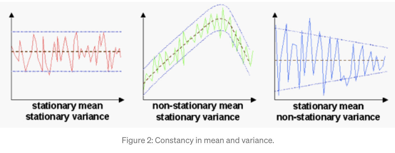
https://towardsdatascience.com/stationarity-in-time-series-analysis-90c94f27322}

Densité spectrale de puissance

• Puissance moyenne

\[P = R_x(0)= E \left[ |x(t)|^2 \right]=\int_{\mathbb{R}} s_x(f)df\]

• Densité spectrale de puissance

  • Définition

  \[s_x(f)=\textrm{TF} \left[ R_x(\tau) \right]\]

  • Propriétés

  \[s_x(f)={\underset{T \rightarrow \infty }{\lim }} \frac{1}{T} E \left[ \left| X_T(f) \right|^2 \right]\]

mais en général \(X(f)\) n’existe pas !

Exemples

• Exemple 1 : Sinusoïde

  \[x(t)= A \cos(2 \pi f_0 t + \theta)\]

  \(\theta\) v.a. uniforme sur \([0, 2\pi]\).

  • Fonction d’autocorrélation

    \[R_x(\tau)=\frac{A^2}{2} \cos(2 \pi f_0 \tau)\]

  • Densité spectrale de puissance

    \[s_x(f)=\frac{A^2}{4} \left[ \delta(f-f_0) + \delta(f+f_0)\right]\]

Exemples

• Exemple 2 : Bruit blanc

  • Fonction d’autocorrélation

    \[R_x(\tau)= \frac{N_0}{2} \delta(\tau)\]

  • Densité spectrale de puissance

    \[s_x(f)= \frac{N_0}{2}\]

Plan du cours

• Chapitre 1 : Corrélations et Spectres

  • Transformée de Fourier

  • Classes de signaux déterministes et aléatoires

  • Propriétés de \(R_x(\tau)\) et de \(s_x(f)\)

• Chapitre 2 :Filtrage Linéaire

• Chapitre 3 : Traitements Non-linéaires

Propriétés de \(R_x(\tau)\)

• Symétrie Hermitienne : \(R_x^*(-\tau)= R_x(\tau)\)

• Valeur maximale : \(|R_x(\tau)| \le R_x(0)\)

• Distance entre \(x(t)\) et \(x(t-\tau)\) : si \(x(t)\) est un signal réel

  \[d^2\left[ x(t), x(t-\tau) \right]= 2 \left[ R_x(0) - R_x(\tau)\right]\]

  donc \(R_x(\tau)\) mesure le lien entre \(x(t)\) et \(x(t-\tau)\).

• Décomposition de Lebesgue : dans la quasi-totalité des applications, on a

  \[R_x(\tau) = R_1(\tau) + R_2(\tau)\] où \(R_1(\tau)\) est une somme de fonctions périodiques et \(R_2(\tau)\) tend vers \(0\) lorsque \(\tau \rightarrow \infty\).

Propriétés de \(s_x(f)\)

• DSP réelle :

  \[s_x(f) \in \mathbb{R}\]

  De plus, si \(x(t)\) signal réel, \(s_x(f)\) réelle paire

• Positivité : \(s_x(f) \ge 0\)

• Lien entre DSP et puissance/énergie :

  \[P \; \textrm{ou} \; E = R_x(0) = \int_\mathbb{R} s_x(f) df\]

• Décomposition :

  dans la plupart des applications, on a \(s_x(f) = s_1(f) + s_2(f)\), où \(s_1(f)\) est un spectre de raies et \(s_2(f)\) un spectre continu (cas général : partie singulière).

Que faut-il savoir ?

• Reconnaître si un signal est à énergie finie, à puissance finie périodique ou aléatoire.

• Qu’est ce qu’un signal aléatoire stationnaire ?

• Les différentes définitions d’une fonction d’autocorrélation\(R_x(\tau)\)

• La définition unifiée d’une densité spectrale : \(s_x(f)\) = ?

• Les différentes définitions d’une densité spectrale

• Ce qu’est un bruit blanc

• Ce qu’est un bruit gaussien

• Propriétés de \(R_x(\tau)\)

• Propriétés de \(s_x(f)\)

Plan du cours

• Chapitre 1 : Corrélations et Spectres

• Chapitre 2 :Filtrage Linéaire

  • Introduction

  • Relations de Wiener-Lee

  • Formule des interférences

  • Exemples

• Chapitre 3 : Traitements Non-linéaires

Introduction

On cherche une opération avec les propriétés suivantes

• Linéarité : \(T\left[ a_1 x_1(t) + a_2 x_2(t) \right] = a_1 T\left[ x_1(t) \right]+ a_2 T\left[x_2(t) \right]\)

• Invariance dans le temps :

  Si \(y(t) = T\left[ x(t) \right]\) alors \(T\left[ x(t-t_0) \right] = y(t-t_0)\)

• Stabilité BIBO :

  Si \(|x(t)| \le M_x\) alors il existe \(M_y\) tel que

  \[|y(t)| =|T\left[x(t) \right]| \le M_y\]

• ``Limitation’’ du spectre d’un signal :

☞ Convolution

\[y(t)= x(t) * h(t) = \int_\mathbb{R} x(u)h(t-u)du = h(t) * x(t)\]

ECG avant filtrage

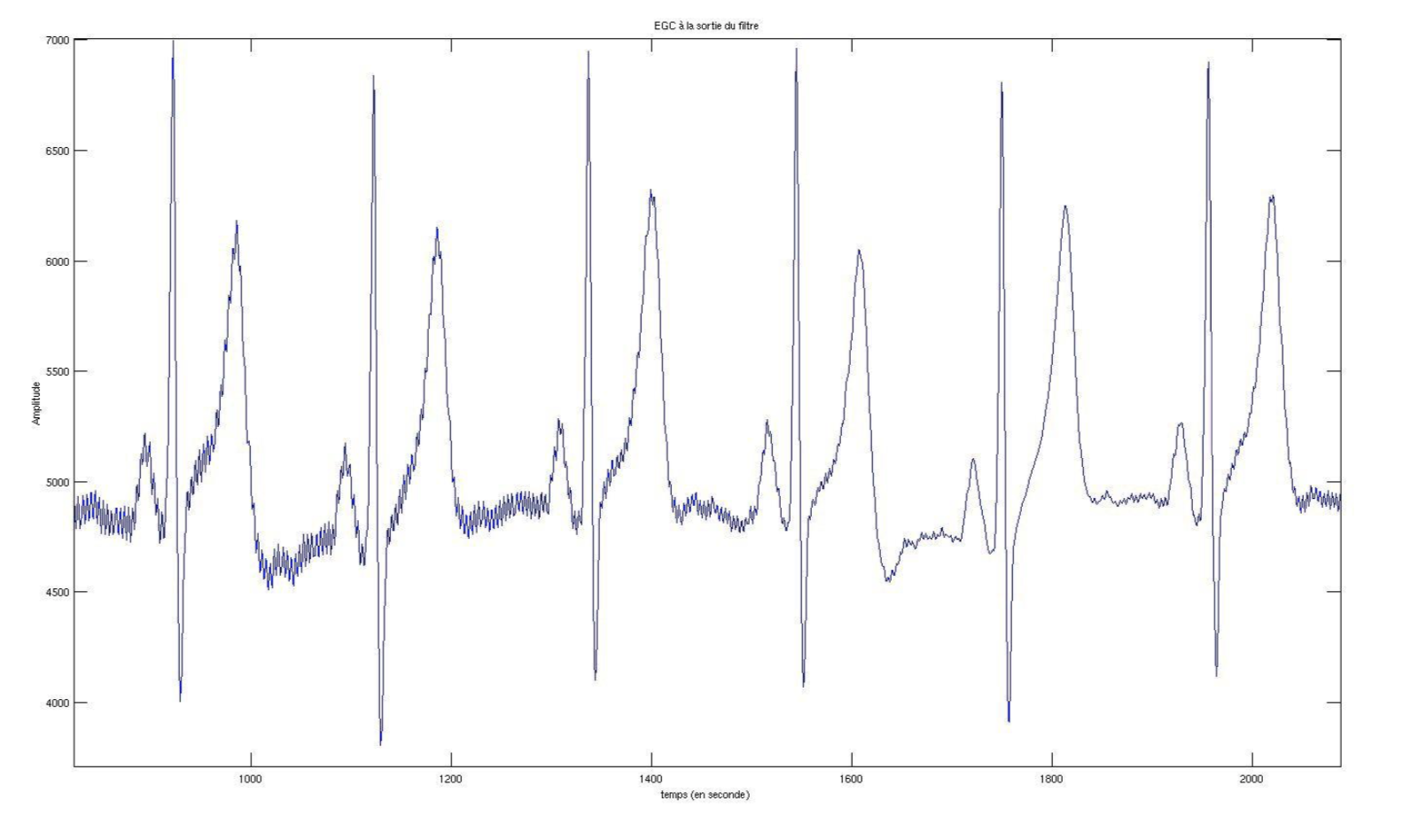
ECG après filtrage

Commentaires

• La linéarité ne suffit pas. Contre-exemple

\[y(t) =m(t)x(t)\]

• CNS de Stabilité BIBO

\[\int_\mathbb{R} |h(t)| dt < \infty, \textrm{i.e.}, h \in L^1\]

• Réponse impulsionnelle et Transmittance

\[H(f)=\textrm{TF} \left[ h(t) \right]=\int_\mathbb{R} h(t) \exp (-j 2 \pi f t) dt\]

Si \(x(t)=\delta(t)\) alors \(y(t)=h(t)\). Ceci permet d’obtenir la seule réponse impulsionnelle possible.

Réalisabilité d’un filtre

• Domaine temporel

  1. \(h(t)\) réelle

  2. \(h(t) \in L^1\) (stabilité )

  3. \(h(t)\) causale (filtre sans mémoire)

• Domaine spectral

  1. Symétrie hermitienne : \(H^*(-f)=H(f)\)

  2. Ne peut se traduire

  3. \(H(f) = -j \widetilde{H}(f)\), où \(\widetilde{H}(f) = H(f)* \frac{1}{\pi f}\) est la transformée de Hilbert de \(H\) (preuve dans le cours manuscrit).

Ecriture équivalente

En écrivant \(H(f)=H_r(f)+jH_i(f)\), on obtient

\[ \begin{aligned} H_r(f)=& H_i(f) *\frac{1}{\pi f} \\ H_i(f)=& - H_r(f) *\frac{1}{\pi f} \end{aligned} \]

Identifier une relation de filtrage linéaire

• Signaux déterministes

  \[y(t)= x(t)*h(t) \; \Leftrightarrow \; Y(f)= X(f) H(f)\]

• Signaux aléatoires : Isométrie fondamentale

  \[\textrm{Si} \; x(t) \; \overset{{I}}{{ \leftrightarrow}} \; e^{j 2 \pi f t}, \; \textrm{alors} \; y(t) \; \overset{{I}}{{\leftrightarrow}} \; e^{j 2 \pi f t} H(f)\]

• Exemples

  • \(y(t) = \sum_{k=1}^n a_k x(t-t_k)\)

  • \(y(t)=x'(t)\)

  • \(y(t)=x(t)m(t)\)

Plan du cours

• Chapitre 1 : Corrélations et Spectres

• Chapitre 2 :Filtrage Linéaire

  • Introduction

  • Relations de Wiener-Lee

  • Formule des interférences

  • Exemples

• Chapitre 3 : Traitements Non-linéaires

Relations de Wiener Lee

• Densité spectrale de puissance

\[s_y(f)=s_x(f) |H(f)|^2\]

• Intercorrélation

\[R_{yx}(\tau)=R_x(\tau) * h(\tau)\]

• Autocorrélation

\[R_y(\tau) = R_x(\tau) * h(\tau) * h^*(-\tau)\]

Preuves (signaux à énergie finie)

• Densité spectrale de puissance

\[s_y(f)=|Y(f)|^2 = |X(f)H(f)|^2 = s_x(f) |H(f)|^2\]

• Intercorrélation

\[\begin{aligned} R_{yx}(\tau)=&\int_\mathbb{R} y(u)x^*(u - \tau)du \\ =& \int_\mathbb{R} Y(f)\left[ e^{-j2 \pi f \tau} X(f) \right]^* df\\ =&\int_\mathbb{R} X(f) H(f) \left[ e^{j 2 \pi f \tau} X^*(f)\right]df\\ =&\int_\mathbb{R} s_x(f) H(f) e^{j 2 \pi f \tau} df =\textrm{TF}^{-1} [s_x(f) H(f)] \quad \textrm{CQFD} \end{aligned}\]

Preuve (signaux à puissance finie)

• Intercorrélation

\[\begin{align*} R_{yx}(\tau)=& \frac{1}{T_0} \int_{-T_0/2}^{T_0/2} y(t)x^*(t-\tau)dt \\ =& \frac{1}{T_0} \int_{-T_0/2}^{T_0/2} \left[\int_\mathbb{R} h(v) x(t-v)dv \right] x^*(t-\tau)dt \\ =&\int_\mathbb{R} h(v) \left[ \frac{1}{T_0} \int_{-T_0/2}^{T_0/2} x(t-v) x^*(t-\tau)dt \right] dv\\ =&\int_\mathbb{R} h(v) R_x(\tau - v)dv \quad \textrm{CQFD} \end{align*}\]

• etc…

Preuves (signaux aléatoires)

• Intercorrélation

\[\begin{align*} R_{yx}(\tau)=& E[ y(t)x^*(t-\tau)] \\ =& \langle y(t), x(t-\tau) \rangle \\ =& \langle e^{j2 \pi ft} H(f) , e^{j2 \pi f(t-\tau)} \rangle\\ =&\int_\mathbb{R} e^{j2 \pi ft} H(f)e^{-j2 \pi f(t-\tau)} s_X(f) df \\ =&\int_\mathbb{R} H(f)e^{j2 \pi f \tau} s_X(f) df \\ =& \; h(\tau) * R_x(\tau) \quad \textrm{CQFD} \end{align*}\]

Preuves (signaux aléatoires)

• Autocorrélation

\[\begin{align*} R_{y}(\tau)=& E[ y(t)y^*(t-\tau)] \\ =& \langle y(t), y(t-\tau) \rangle \\ =& \langle e^{j2 \pi ft} H(f) , e^{j2 \pi f(t-\tau)} H(f) \rangle\\ =&\int_\mathbb{R} e^{j2 \pi ft} H(f)e^{-j2 \pi f(t-\tau)} H^*(f) s_x(f) df \\ =&\int_\mathbb{R} |H(f)|^2 s_x(f) e^{j2 \pi f \tau} df \\ =& \textrm{TF}^{-1} \{ s_x(f) |H(f)|^2 \} \\ =& \; h(\tau) * h^*(-\tau) * R_x(\tau) \quad \textrm{CQFD} \end{align*}\]

Preuves (signaux aléatoires)

• Autocorrélation

\[R_{y}(\tau)= \textrm{TF}^{-1} \{ s_x(f) |H(f)|^2 \}\]

• Densité Spectrale de Puissance

\[s_y(f)=s_x(f) |H(f)|^2 \quad \textrm{CQFD}\]

Valeur moyenne

• Propriété

\[E[Y(t)]=E[X(t)] H(0)\]

• Preuve

\[\begin{align*} E[Y(t)]=& E\left[ \int_\mathbb{R} X(t-u)h(u)du \right] \\ =& \int_\mathbb{R} E[X(t-u)] h(u)du \\ =& E[X(t)] \int_\mathbb{R} h(u)du \quad \textrm{(signal stationnaire)}\\ =& E[X(t)] H(0) \quad \textrm{CQFD} \end{align*}\]

Plan du cours

• Chapitre 1 : Corrélations et Spectres

• Chapitre 2 :Filtrage Linéaire

  • Introduction

  • Relations de Wiener-Lee

  • Formule des interférences

  • Exemples

• Chapitre 3 : Traitements Non-linéaires

Formule des interférences

• Hypothèses

\[y_1(t)= x(t)*h_1(t) \; \textrm{et} \; y_2(t)= x(t)*h_2(t)\]

• Conclusion

\[R_{y_1 y_2}(\tau) = \int_\mathbb{R} s_x(f) H_1(f) H_2^*(f) e^{j 2\pi f \tau} df\]

Preuve (signaux à énergie finie)

\[\begin{align*} R_{y_1 y_2}(\tau)&= \int y_1(t) y_2^*(t-\tau) dt =\int_\mathbb{R} Y_1(f) \left[ Y_2(f) e^{-j 2 \pi f \tau} \right]^* df \\ & = \int_\mathbb{R} H_1(f) H_2^*(f) e^{j 2 \pi f \tau} s_x(f) df \quad \textrm{CQFD} \end{align*}\]

Plan du cours

• Chapitre 1 : Corrélations et Spectres

• Chapitre 2 :Filtrage Linéaire

  • Introduction

  • Relations de Wiener-Lee

  • Formule des interférences

  • Exemples

• Chapitre 3 : Traitements Non-linéaires

Exemples

• Filtre Passe-bas

  • Transmittance

  \[H(f)= \Pi_F(f)\]

  • Réponse impulsionnelle

  \[h(t)= F \textrm{sinc} \left( \pi F t \right)\]

  non causale et \(\notin L^1 \; \Rightarrow \;\) troncature + décalage

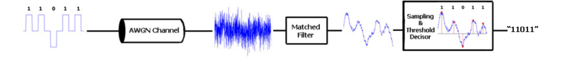
• Filtres liaisons montante et descendante d’une chaîne de transmission

Filtre adapté : maximisation du SNR

• Signal observé

\[x(t)=s(t)+n(t),\qquad t\in \left[ 0,T\right] \]

\(s(t)\) signal déterministe à énergie finie et \(n(t)\) signal aléatoire stationnaire de moyenne nulle et de densité spectrale de puissance \(s_n(f)\).

• Filtrage

\[y(t) =y_{s}(t)+y_{n}(t) =s(t)\ast h(t)+n(t)\ast h(t)\]

• Rapport signal sur bruit à l’instant \(t=t_0\)

\[\text{SNR}(t_{0})=\frac{y_{s}^{2}(t_{0})}{E\left[ y_{n}^{2}(t_{0})\right] }\]

Expression équivalente du SNR

\[SNR(t_{0})=\frac{y_{s}^{2}(t_{0})}{E\left[ y_{n}^{2}(t_{0})\right] }=\frac{\left| \int_{\Bbb{R}}H(f)S(f)e^{j2\pi ft_{0}}df\right|^{2}}{\int_{\Bbb{R}}\left| H(f)\right| ^{2}s_{n}(f)df} \]

• Numérateur

\[y_{s}(t)=TF^{-1}\left[ S(f)H(f)\right] =\int_{\Bbb{R}}H(f)S(f)e^{j2\pi ft}df\]

• Dénominateur

  • Wiener Lee

  \[s_{y_{n}}(f)=s_{n}(f)\left| H(f)\right| ^{2}\]

  • Puissance

  \[P_{y_{n}} =E\left[ y_{n}^{2}(t_{0})\right] =R_{y_{n}}\left( 0\right)=\int_{\Bbb{R}}s_{n}(f)\left| H(f)\right| ^{2}df\]

Inégalité de Cauchy-Schwartz

\[\left| \int_{\Bbb{R}}a(f)b^{\ast }(f)df\right| ^{2}\leq \int_{\Bbb{R}}a(f)a^{\ast }(f)df\int_{\Bbb{R}}b(f)b^{\ast }(f)df\]

• Numérateur

\[\left| \int_{\Bbb{R}}H(f)S(f)e^{j2\pi ft_0}df\right|^2 = \left| \int_{\Bbb{R}}a(f)b^{\ast }(f)df\right| ^{2}\]

avec \(a(f)=\sqrt{s_{n}(f)}H(f)\) et \(b(f)=\frac{S^{\ast }(f)}{\sqrt{s_{n}(f)}}e^{-j2\pi ft_{0}}\).

• Dénominateur

\[\int_{\Bbb{R}}s_{n}(f)\left| H(f)\right| ^{2}df = \int_{\Bbb{R}}a(f)a^{\ast }(f)df\]

Expression du filtre adapté

• Cauchy-Schwartz

\[SNR(t_{0})=\frac{\left| \int_{\Bbb{R}}H(f)S(f)e^{j2\pi ft_{0}}df\right| ^{2}}{\int_{\Bbb{R}}\left| H(f)\right| ^{2}s_{n}(f)df} \le \int_{\Bbb{R}}b(f)b^{\ast }(f)df\] avec égalité pour \(a(f)= k b(f)\), i.e.,

\[H(f)=k\dfrac{S^{\ast }(f)}{s_{n}(f)}e^{-j2\pi ft_{0}}\]

• Cas d’un bruit blanc

\[H(f)=KS^{\ast }(f)e^{-j2\pi ft_{0}} \Leftrightarrow h(t)=Ks^{\ast }\left( t_{0}-t\right)\] Symétrie oy + Translation

SNR maximum

• Définition

\[SNR(t_{0})^{\max } =\int_{\Bbb{R}}b(f)b^{\ast }(f)df =\int_{\Bbb{R}}\frac{2}{N_{0}}\left| S(f)\right| ^{2}df=\frac{2E}{N_{0}}\] où \(E\) est l’énergie du signal. On voit donc que le le rapport signal à bruit maximal ne dépend pas de la forme du signal mais uniquement de son énergie.

• Page wikipedia Matched Filter

Que faut-il savoir ?

• Reconnaître une relation de filtrage linéaire.

• Densité spectrale de puissance de la sortie d’un filtre

• Intercorrélation entre l’entrée et la sortie d’un filtre

• Moyenne de la sortie d’un filtre

• Formule des interférences

• Réponse impulsionnelle causale et \(\in \mathcal{L}^1\) , sinon…

Plan du cours

• Chapitre 1 : Corrélations et Spectres

• Chapitre 2 :Filtrage Linéaire

• Chapitre 3 : Traitements Non-linéaires

  • Introduction
  • Quadrateur
  • Quantification

Introduction

• Transformation sans mémoire

\[y(t)= g \left[ x(t) \right]\]

• Exemples

  • Quadrateur

  \[y(t) = x^2 (t)\]

  • Quantification

  \[y(t) = x_Q (t)\]

Plan du cours

• Chapitre 1 : Corrélations et Spectres

• Chapitre 2 :Filtrage Linéaire

• Chapitre 3 : Traitements Non-linéaires

  • Introduction
  • Quadrateur
  • Quantification

Quadrateur

• Signaux déterministes

\[Y(f) = X(f) * X(f)\]

• Exemples

  • Sinusoïde : \(x(t) = A \cos (2 \pi f_0 t)\)

  \[Y(f) =\frac{A^2}{2} \delta(f) + \frac{A^2}{4} \left[\delta(f-2f_0)+ \delta(f+2 f_0) \right]\]

  Disparition de la fréquence \(f_0\) et apparition de la fréquence \(2 f_0\)

  • Somme de sinusoïdes : Termes d’intermodulation

  • Sinus cardinal : doublement de la largeur de bande

Signal aléatoire gaussien

• Définition

  On dit qu’un signal aléatoire \(X(t)\) est gaussien si pour tout ensemble d’instants \((t_1,...,t_n)\), le vecteur \(\left[ X(t_1),...,X(t_n) \right]^T\) est un vecteur gaussien de \(\mathbb{R}^n\).

• Loi univariée de \(X(t)\)

  La loi de \(X(t)\) est alors une loi gaussienne de densité

  \[p[X(t)]=\frac{1}{\sqrt{2 \pi \sigma^2(t)}} \exp \left\{ - \frac{\left[ X(t) - m(t) \right]^2 }{2 \sigma^2(t)} \right\}.\]

  Si le signal \(X(t)\) est stationnaire au sens large alors

  \[m(t)=E[X(t)]=m, \; \text{et} \; \sigma^2(t)=E[X^2(t)] - E^2[X(t)]=R_X(0)-m^2.\]

  donc les paramètres de la densité de \(X(t)\) sont indépendants du temps.

Signal aléatoire gaussien

• Loi bivariée de \([X(t), X(t-\tau)]\)

  La loi du vecteur \(\boldsymbol{V}(t)=[X(t), X(t-\tau)]^T\) est alors une loi gaussienne de \(\mathbb{R}^2\) de densité

  \[p[x(t),x(t-\tau)]=\frac{1}{2 \pi \sqrt{|\boldsymbol{\Sigma}(t)|}} \exp \left\{ - \frac{1}{2} \left[ \boldsymbol{V}(t) - \boldsymbol{m}(t) \right]^T \boldsymbol{\Sigma}^{-1}(t) \left[ \boldsymbol{V}(t) - \boldsymbol{m}(t) \right]\right\}.\]

  où \(\boldsymbol{m}(t)=[ m_1(t), m_2(t) ]^T \in \mathbb{R}^2\) est le vecteur moyenne, avec \(m_1(t)= E[X(t)]\) et \(m_2(t)=E[X(t-\tau)]\), et \(\boldsymbol{\Sigma}(t) \in \mathcal{M}_2(\mathbb{R})\) est la matrice de covariance définie par

  \[\boldsymbol{\Sigma}(t) = \left( \begin{array}{ll} \sigma_1^2(t,\tau) & \sigma_{1,2}(t,\tau) \\ \sigma_{1,2}(\tau) & \sigma_2^2(t, \tau) \end{array} \right)\]

où \(\sigma_1^2(t,\tau)\) et \(\sigma_2^2(t,\tau)\) sont les variances de \(X(t)\) et de \(X(t-\tau)\) et \(\sigma_{1,2}(t,\tau)\) est la covariance \([ X(t), X(t-\tau)]^T\). Si le signal \(X(t)\) est stationnaire au sens large alors

\[\sigma_{i}(t,\tau)= R_X(0)-m^2 \; \text{et} \; \sigma_{1,2}(t,\tau)=E[X(t)X(t-\tau)] - E[X(t)] E[X(t-\tau)]=R_X(\tau)-m^2.\]

donc les paramètres de la densité de \(\boldsymbol{V}(t)\) sont indépendants du temps.

Stationnarité de \(Y(t)=g[X(t)]\)

Si \(X(t)\) est un signal aléatoire stationnaire, alors pour toute non-linéarité \(g\), \(Y(t)\) est également un signal aléatoire stationnaire. En effet,

• Moyenne

\[E[Y(t)]=E \left\{ g[X(t)] \right\}=\int g[x(t)] p[x(t)] dx(t).\] Comme les paramètres de \(p[x(t)]\) ne dépendent que de \(R_X(0)\) et de \(m\), \(E[Y(t)]\) est une quantité indépendante de \(t\).

• Fonction d’autocorrélation

\[E\left[ Y(t) Y(t-\tau) \right] = \int \int g[x(t)] g[x(t-\tau)] p[x(t),x(t-\tau)] dx(t) dx(t-\tau).\] Comme les paramètres de \(p[x(t), x(t-\tau)]\) ne dépendent que de \(R_X(\tau)\), \(R_X(0)\) et de \(m\), \(E[Y(t)Y(t-\tau)]\) est une quantité indépendante de \(t\).

Le signal \(Y(t)\) est donc stationnaire au sens large. Sa moyenne dépend de \(R_X(0)\) et de \(m\) et sa fonction d’autocorrélation dépend de \(R_X(\tau)\), \(R_X(0)\) et de \(m\).

Quadrateur pour signaux aléatoires

• Théorème de Price

  • Hypothèses

    \((X_1,X_2)\) vecteur Gaussien de vecteur moyenne nul

    \(Y_1=g(X_1)\) et \(Y_2=g(X_2)\)

  • Conclusion

    \[\frac{\partial E(Y_1 Y_2) }{\partial E(X_1 X_2)} = E \left( \frac{\partial Y_1}{\partial X_1} \frac{\partial Y_2}{\partial X_2} \right)\]

  • Application au quadrateur

    \[R_Y(\tau) = 2 R_X^2(\tau) + K\]

Détermination de \(K\)

• Moments d’une loi Gaussienne centrée

\[E \left( X^{2n+1} \right) = 0 , \; E \left( X^{2n} \right) = [(2n-1)\times (2n-3) ... \times 3 \times 1] \sigma^{2n}\]

• \(\tau=0\)

\[K = R_Y(0) - 2 R_X^2(0) = 3 R_X^2(0) - 2 R_X^2(0) =R_X^2(0)\]

• \(\tau \rightarrow +\infty\)

\[K = R_Y(+ \infty)- 2 R_X(+ \infty) = R_X^2(0) \]

• Autocorréation

\[R_Y(\tau) = 2 R_X^2(\tau) + R_X^2(0)\]

Summary

• Autocorréation

\[R_Y(\tau) = 2 R_X^2(\tau) + R_X^2(0)\]

• Densité spectrale de puissance

\[s_Y(f) = 2 s_X(f) * s_X(f) + R_X^2(0) \delta(f)\]

Plan du cours

• Chapitre 1 : Corrélations et Spectres

• Chapitre 2 :Filtrage Linéaire

• Chapitre 3 : Traitements Non-linéaires

  • Introduction
  • Quadrateur
  • Quantification

Quantification

• Principe :

\[x_Q(t) =i \Delta q_i =x_i \; \textrm{et} \; x_i - \frac{\Delta q_i}{2} \le x(t) \le x_i + \frac{\Delta q_i}{2}\]

• Définitions :

  • Pas de quantification : \(\Delta q_i\)

  • Quantification uniforme : \(\Delta q_i = \Delta q = \frac{2 A_{\max}}{N}\)

  • Niveaux de quantification : \(x_i\)

  • Nombre de bits de quantification : \(N=2^n\)

Erreur de quantification

• Hypothèses :

  \(\epsilon(t)\) suit la loi uniforme sur \(\left[-\frac{\Delta q}{2} , \frac{\Delta q}{2} \right]\), i.e., \(N \ge 2^8\)

• Rapport signal sur bruit de quantification :

  \[\textrm{SNR}_{\textrm{dB}}=10 \log_{10} \left(\frac{\sigma^2_x}{\sigma^2_{\epsilon}}\right)\]

  • Variance du bruit : \(\sigma^2_{\epsilon} = \frac{(\Delta q)^2}{12}\)

  • Sinusoïde : \(\sigma^2_x= \frac{A^2}{2}\)

• Conclusion :

\[\textrm{SNR}_{\textrm{dB}}= 6n + 1.76\]

Remarques

• Généralisation à un signal gaussien :

  \[2 S \sigma = N \Delta q \; \Rightarrow \; \textrm{SNR}_{\textrm{dB}}= 6n + ...\]

• Quantification non uniforme

Que faut-il savoir?

• Traitement non-linéaire : = possibilité de créer de nouvelles fréquences

• Savoir appliquer le théorème de Price. Intérêt ?

• Définition et propriétés de la quantification

• Savoir calculer le rapport signal sur bruit de quantification